Persephone User Guide

Here is an example of connecting physical and genetic maps:

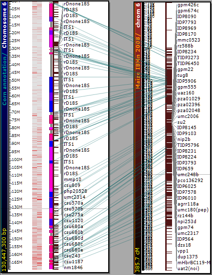
Physical maps for corn also have a track of genetic markers. The position of the markers is based on their sequence and the sequence of corn chromosomes. It is possible, therefore, to calculate an average rate of recombination along the chromosomes by comparing the distance between markers on the physical map and the corresponding genetic map. A colored heat map track shows areas where on average recombination is rare (blue) and regions with high frequency of recombination (red). Usually centromeric regions show much lower recombination rates.

Another way of comparing genetic and physical maps is by mapping the available protein sequences, corresponding to the markers, versus genes predicted on the chromosomes. In this case the marker track on the genetic map will be connected to the gene model track of the physical map.

The plates are connected based on visible tracks. First,Persephone tries to link the genetic map to a marker (heat map) track on the physical map using common marker names. If there are no connectors, it will try to use the gene model track. In this case the marker-gene relations are based on the records in the database.

In case a genetic map is loaded from an external file - which means that there are no internal IDs used - the connection between markers will be done based on marker names. Remember, that markers can have several names but only one of the names is considered the primary name. The other names are regarded as synonyms. The primary marker name is displayed as a label on the map but other synonyms are also used in determining if the markers should be linked.