Use Case
A typical data flow for loading a genome with multiple tracks of annotation that can be linked to other genomes starts with creating an Organism record. All maps should have a reference to an Organism. After that, a Map Set with multiple Maps is created. It can be based on the genomic sequences or genetic linkage groups. Tracks with gene annotation are usually added to the map sets first. Additionally, the maps can have tracks of other types, including quantitative tracks, such as RNA-seq coverage values, marker tracks, QTLs, etc.
This section provides a use case for adding Glycine max (soybean) to your Persephone database using PersephoneShell.
To add soybean genomic data you will need to perform the following tasks:
- Add an Organism
- Download the genomic information for Glycine max. You will need these files for Steps 3, 5, and 6 below. These files should be saved to a location where they can be accessed by PersephoneShell.
- Add a Map Set, Maps, and Sequences
- Optional. Verify Addition of Maps, Map Sets, and Map Set Trees
- Add Gene Annotations
- Add Markers
Tip
If you need to delete any of the data you have loaded, perform the steps outlined in Deleting Loaded Data or to start with an empty database, use the 'init' command to wipe all the data from the database and refresh the schema.
Please also familiarize yourself with Persephone's data hierarchy, which is described below.
Persephone Data Hierarchy
The figure below shows some of the Persephone objects and their relationship.
Data Hierarchy
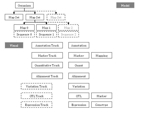
The highest-level model object is Organism which contains taxonomy information, such as scientific name and common name. The corresponding genomic data for Organism can be organized into multiple map sets, which usually represent different assembly builds. A map set consists of chromosomes, scaffolds, or genetic maps, also known as maps. A physical map, such as a chromosome or a scaffold, represents a genomic sequence with features located in base pairs (bp; 1-based), while a genetic map is represented as distances between genetic markers and gene loci in centiMorgan (cM; floating-point numbers).
The mapped features are displayed in a form of tracks. A map can contain multiple tracks of different kinds including
- annotation tracks with gene models,
- marker tracks with SNP markers or repeats,
- quantitative tracks with RNA-seq coverage or methylation profiles,
- variation tracks with multiple genotypes,
- QTL tracks,
- NGS read alignments,
- syntenic blocks,
- tracks with expression data, etc.
 Copyright © 2009-2024 by Persephone Software. All Rights Reserved.