Web Persephone: Multiple Sequence Alignment
Overview
The Multiple Sequence Alignment tool aligns multiple sequences in the same view, generating a consensus alignment. The tool can align protein or DNA sequences, using a selection of different alignment algorithms. You can access the tool from several places: from the Annotation Details dialog (to align protein and DNA sequences of orthologs), from the BLAST Results dialog (to align DNA sequences of HSPs), or from the Tools menu (to align custom sequences).
Orthologs
To generate a multiple alignment for a gene's orthologs, click the gene model to open the Annotation Details dialog; navigate to the Orthologs tab, and click the link in the bottom-right corner of the table: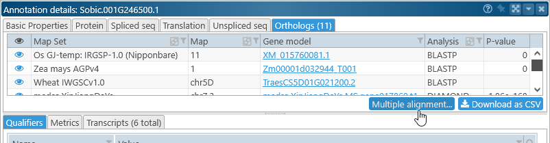
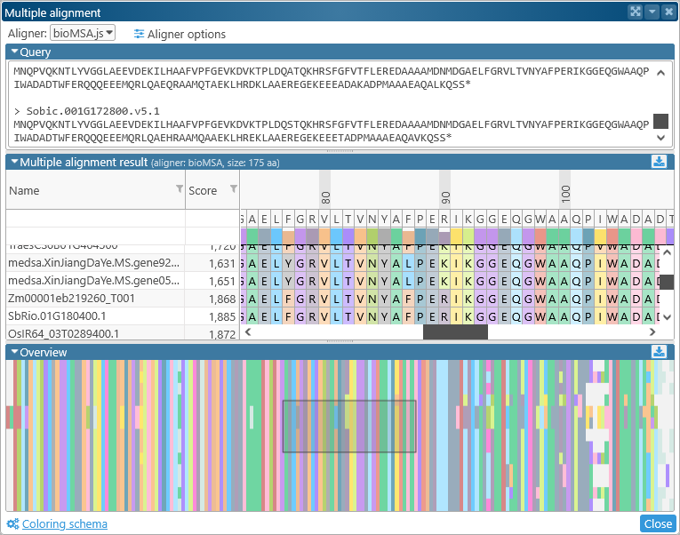
Doing so opens the Multiple Sequence Alignment dialog: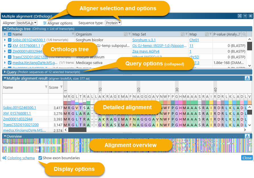
The top part of the dialog contains alignment options and the list of orthologs; the bottom part contains the actual alignment. You can click the  button to expand or collapse each section.
By default, protein sequences for each transcript are aligned, but you can change this using the dropdown menu at the top: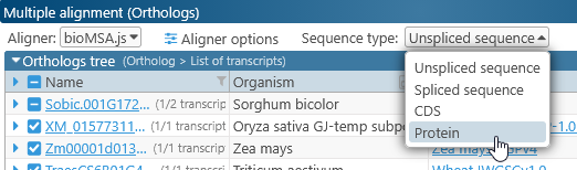
Most of the functionality described below applies to all sequence types, so we will use Protein in this example.
Alignment options
The selection box at the top lists all available alignment algorithms. BioMSA is selected by default; this algorithm is very fast at the expense of some accuracy. Other aligners such as KALIGN or MUSCLE may produce better results, but take longer to run.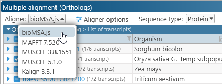
Click the Aligner options button to display specific options for the currently selected aligner. For example, these are the options for BioMSA:
Check the checkboxes next to each option to provide a custom value, or uncheck them to use the defaults.
- Method: Selects the multiple alignment method.
- Auto: Automatically selects the best algorithm based on sequence length. If the total length of the sequences is longer than 30 Kbp, the alignment will be done using the Diag algorithm, otherwise, the Complete algorithm will be used.
- Complete: Performs a more complete alignment (using the Needleman-Wunsch algorithm) at the expense of slower performance.
- Diag: Performs a faster yet less accurate alignment by finding common segments between sequences (called "diagonals"), then running the Needleman-Wunsch algorithm for the missing sequence fragments.
- Gap penalties: Adjusts the gap open penalty and the gap extend penalty for the alignment algorithm. Higher values penalize gaps more severely; lower values allow for more gaps and/or longer gaps.
The Gap penalties in particular are very useful for fine-tuning the alignment; some other algorithms also provide a way to adjust them. For example, here are the options for KALIGN:
Also note that the long textbox at the top of the options popup allows you to enter command-line arguments directly.
Selecting orthologs
The tree view in the top half of the dialog displays all the orthologs available for alignment.
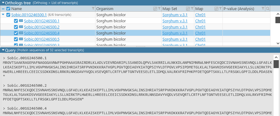
By default, only the representative transcript for each ortholog is included in the comparison; however, you can click the  button to expand the list of available transcripts. The very first item on the list is the currently selected gene, which may also possess multiple transcripts:
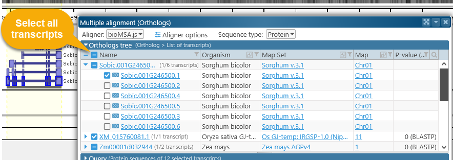
Check the checkbox next to a transcript to add it to the comparison. You can also click the checkbox in the table's header to quickly select all available transcripts, although doing so may cause the alignment calculation to run significantly slower (depending on the number of selected transcripts). Note that the number of selected and available transcripts is listed next to each gene.
Click the name of a transcript to open its Annotation Details dialog: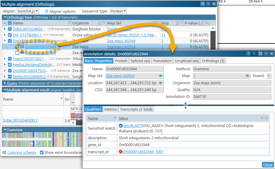
In addition, when you mouse over the name of a transcript, a settings button  will appear:
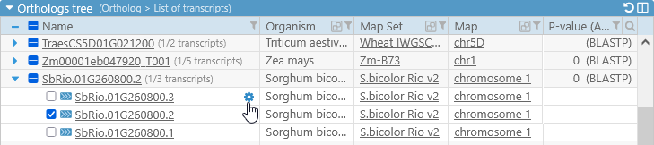
Click the button to choose which label should be shown for all transcripts in the current map set (in this example, Zea Mays AGPv4). By default, the best label is selected automatically; however, you can also choose to manually select the value of any available qualifier:
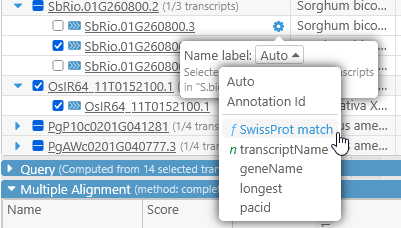
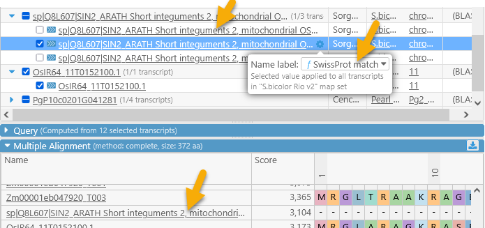
Qualifiers that are marked with "f" contain the gene function, and those marked with "n" contain the gene name; note that these could be different for every map set. The updated label will be reflected in the table as well as the alignment section:
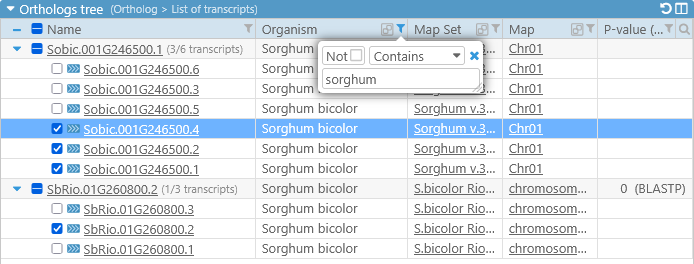
The table of orthologs supports all of the standard search and filtering controls; for example, you could filter the orthologs by organism, hiding all except those that occur on Sorghum (remember to deselect all sequences before filtering):
Sorting the table will also change the sort order of transcript in the alignment sections.
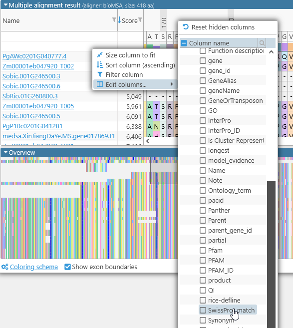
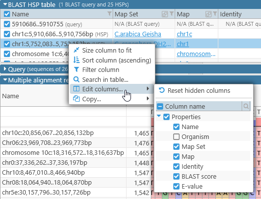
In addition, you can show or hide extra columns by right-clicking anywhere in the table, and selecting Edit columns from the popup menu. For example, you could display the value of the "SwissProt match" qualifier and/or hide the P-value column:
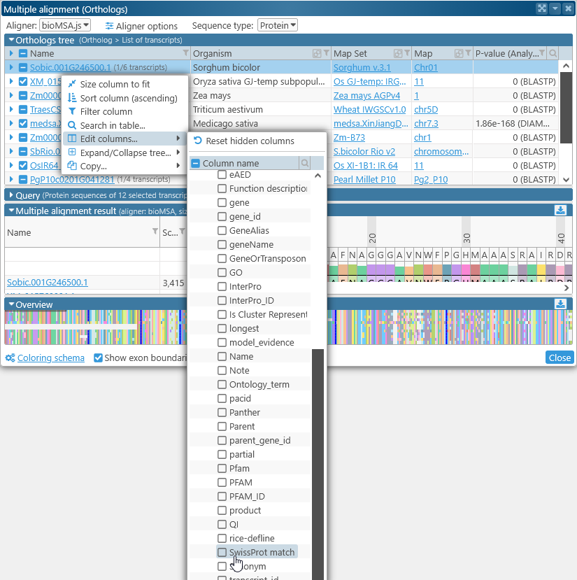
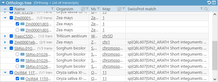
Note that not all qualifiers may be available for all map sets or tracks (in this case, the "SwissProt match" qualifier is not available for some Zea mays map sets). If you have a data file with additional annotation qualifiers, you can load it in PersephoneShell.
Query
The Query section lists all the sequences to be aligned (in this case, selected protein translations of ortholog transcripts), in multi-FASTA format:
The query is read-only in this mode, but will become editable if you open the Multiple Sequence Alignment tool manually (as described below).
Alignment result display and Overview
The middle portion of the dialog displays the detailed sequence alignment; the bottom portion displays the "bird's eye" overview. The overview compresses the entire alignment to fit on the screen, making it easier to find gaps or blocks of mismatches: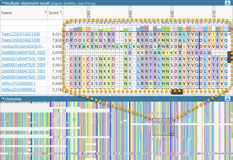
Drag the mouse over the overview to quickly scroll the main alignment display to the desired position. The leftmost two columns in the main alignment view display the name of each aligned transcript and its multiple alignment match score (higher scores indicate a better match to the consensus alignment). You can resize these columns by dragging their borders (as with any table in Persephone). You may also find it useful to sort the transcripts by score, as doing so sometimes produces a more legible picture: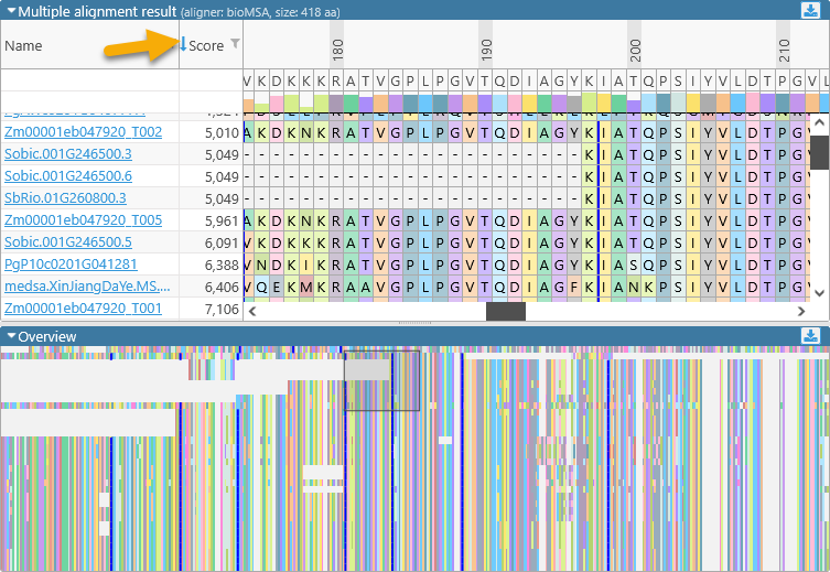
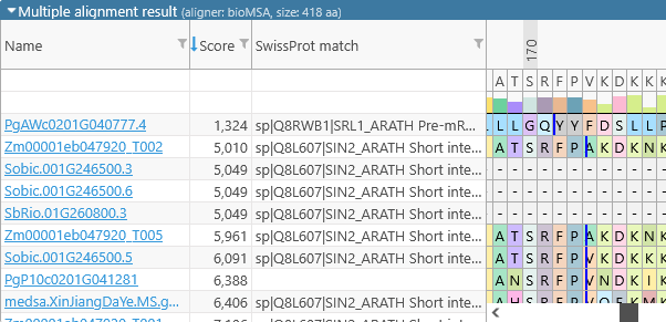
In addition, you can right-click inside any of these columns to bring up the Edit columns menu. For example, you can use it to display the value of the "SwissProt match" qualifier in each alignment line:
The numbers above the amino acids display their position (in amino acids) relative to the start of the consensus alignment. The consensus alignment itself is displayed at the top, along with the bar chart showing the prevalence of the most common amino acid at each position in the consensus. Mouse over any amino acid to display a popup balloon with more information: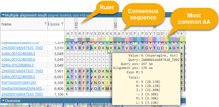
As in many Persephone tables, a click on a column header (in this case, the position) will sort the cells based on the values in the clicked column.
The thick blue lines (in the main alignment view as well as the bird's-eye overview) represent exon boundaries of the gene that produced the transcript, although you can turn them off: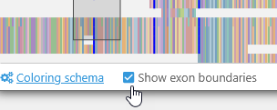
You can click a transcript name to display its Annotation Details, or mouse over it and click the button to display its settings:
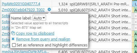
In this popup, you can change the displayed label for the transcript (the same way as in the main table), and perform some additional functions:
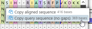
- Copy row to clipboard: Copies the selected alignment row to the clipboard, including gaps (represented by dashes). To copy just the aligned sequence without the gaps, right click its row and choose the appropriate option:
- Remove from query and realign: Removes this transcript from the query and re-runs the currently selected aligner. If you chose this option by mistake, you can always re-select the transcript in the main table.
- Set as reference and highlight differences: By default, all amino acids are highlighted with their individual colors; but you can use this option to set the selected transcript as reference, and highlight only those amino acids that are different from it. These highlighting options are described in more detail below.
Display options
You can fine-tune the color-coding scheme for the amino acids by opening the Coloring schema panel: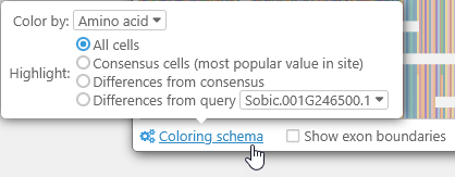
- Color by:
- Amino acid: This is the default option; each kind of amino acid is highlighted with its own unique color. Likewise, when aligning DNA sequences, each base is highlighted in its own color (just as they are on the GC-Content track).
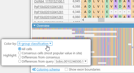
- R-Group classification: Highlights amino acids by their side chain types.
- Highlight:
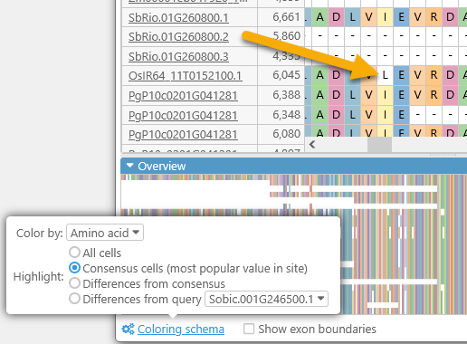
- All cells: By default, all amino acids (or bases) are highlighted (as per the Color by selection).
- Consensus cells: Highlights only those amino acids that match the consensus alignment; for example, this Leucine is not highlighted because most of the transcripts contain Isoleucine at its position:
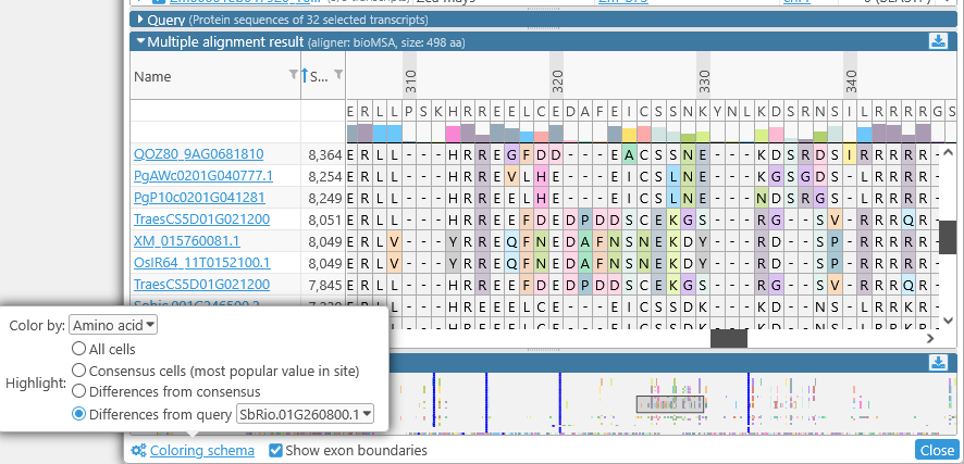
- Differences from consensus: The opposite of the above; highlights only those amino acids that differ from the consensus alignment.
- Differences from query: You can nominate one transcript to act as the reference, and highlight only those amino acids that differ from it. For example, you could highlight the differences from SbRio.01G260800.1 among all of the other Sorghum transcripts:
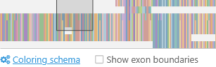
You can also turn off the thick blue lines representing exon boundaries:
Note
Exon boundaries are not available when aligning Unspliced sequences.
Exporting alignments
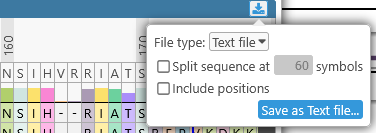
Click the  button in the upper-right corner of the detailed alignment view to export it, either as an SVG image (suitable for publication), or as plain text. You can choose whether to split the alignment lines by width, and also whether to include relative position labels:
Method: complete, Gap open penalty: -300, Gap extend penalty: -11, Queries: 9, Size: 369 aa
1
SbRio.01G260800.1 MRGVTSAAKRAGEMAFNAGGGAVNWFPGHMAAASRAIRDRLKLADLVIEVRDARIPLSSA
SbRio.01G260800.2 ------------------------------------------------------------
SbRio.01G260800.3 ------------------------------------------------------------
Sobic.001G246500.1 MRGVTSAAKRAGEMAFNAGGGAVNWFPGHMAAASRAIRDRLKLADLVIEVRDARIPLSSA
Sobic.001G246500.2 ------------------------------------------------------------
Sobic.001G246500.3 ------------------------------------------------------------
Sobic.001G246500.4 ------------------------------------------------------------
Sobic.001G246500.5 ------------------------------------------------------------
Sobic.001G246500.6 ------------------------------------------------------------
61
SbRio.01G260800.1 NEDLQPVLSAKRRILALNKKDLANPNIMNRWLNHFESCKQDCISVNAHSSNSVNQLLGFA
SbRio.01G260800.2 ---------------------------MNRWLNHFESCKQDCISVNAHSSNSVNQLLGFA
SbRio.01G260800.3 ----------------------------------MESGKMSSHPAQQKKLSSLT------
Sobic.001G246500.1 NEDLQPVLSAKRRILALNKKDLANPNIMNRWLNHFESCKQDCISVNAHSSNSVNQLLGFA
Sobic.001G246500.2 ---------------------------MNRWLNHFESCKQDCISVNAHSSNSVNQLLGFA
Sobic.001G246500.3 ----------------------------------MESGKMSSHPAQQKKLSSLT------
Sobic.001G246500.4 ---------------------------MNRWLNHFESCKQDCISVNAHSSNSVNQLLGFA
Sobic.001G246500.5 ------------------------------------------------------------
Sobic.001G246500.6 ----------------------------------MESGKMSSHPAQQKKLSSLT------
...
You can also export the bird's-eye overview of the entire alignment in SVG vector format, suitable for publication.
BLASTN results
To align DNA sequences from BLASTN results, first run a BLAST search as usual; then select relevant hits, and click the Multiple alignment button in the BLAST Results dialog. For example, you could BLAST an assay sequence against several varieties of Coffee in search of a primer position:

Doing so produces multiple hits across the Coffee varieties:
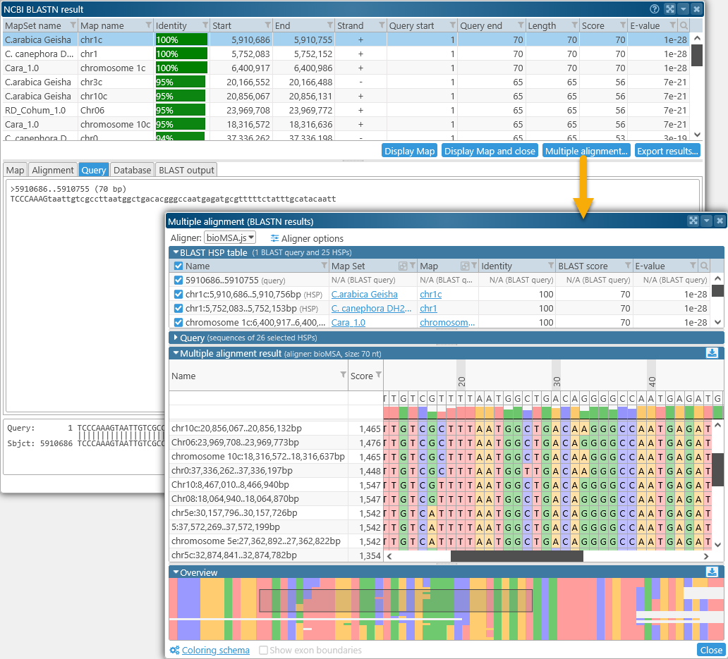
DNA multiple alignment functions similarly to protein multiple alignment, with a few minor differences.
- The sequences being aligned are individual BLAST HSPs, i.e. DNA segments that had a good match on one of the target genomes. The original BLAST query is listed at the top:

The HSPs are given auto-generated names based on their hit location. - The list of available columns is different, containing the properties of each HSP as provided by BLAST:
- The Show exon boundaries option is not available (since only the individual HSPs are being aligned, not entire transcripts).
- You can select a region of the alignment to calculate the melting temperature for each aligned sequence inside the selection. To do so, click and drag on the alignment to draw a bounding box around the region of interest:
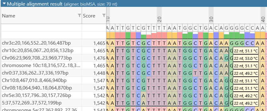
The melting temperature for each sequence fragment within the bounding box is shown in the yellow tooltip on the right-hand side. This melting temperature is approximated using the basic Tm formula, e.g. as described here (or here):
Two standard approximation calculations are used.
• For sequences less than 14 nucleotides the formula is:
Tm= (wA+xT) * 2 + (yG+zC) * 4
where w,x,y,z are the number of the bases A,T,G,C in the sequence, respectively.
• For sequences longer than 13 nucleotides, the equation used is
Tm= 64.9 +41*(yG+zC-16.4)/(wA+xT+yG+zC)
Custom alignment
To align custom sequences, select Multiple alignment from the Tools menu on the main toolbar: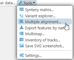
Doing so will open a blank Multiple alignment dialog, with the Query box expanded. Paste your desired query (in multi-FASTA format) into this box to generate the alignment:
The sequence type (DNA or Protein) will be auto-detected based on the sequences you pasted; the name of each sequence will be taken from its FASTA header. In this mode, no additional columns (besides Name and Score) are available, but all other functionality is available as normal. As you edit the query, the changes you make will be automatically reflected in the alignment.
 Copyright © 2009-2025 by Persephone Software. All Rights Reserved.